As-of vs. as-was: bitemporal modeling for financial reporting

TL;DR

• Every financial fact needs two timestamps: when it happened (effective_at) and when the warehouse learned about it (recorded_at).
• As-of is today's best knowledge of a past date; as-was is what you published at close. Finance needs both, and every chart must say which one it shows.
• Keep facts append-only, version dimensions on system time, and freeze each close as an immutable snapshot that published reports read from.
• A restatement bridge explains every difference by cause, so a $6,600 gap becomes a late deposit plus a price correction instead of a mystery.

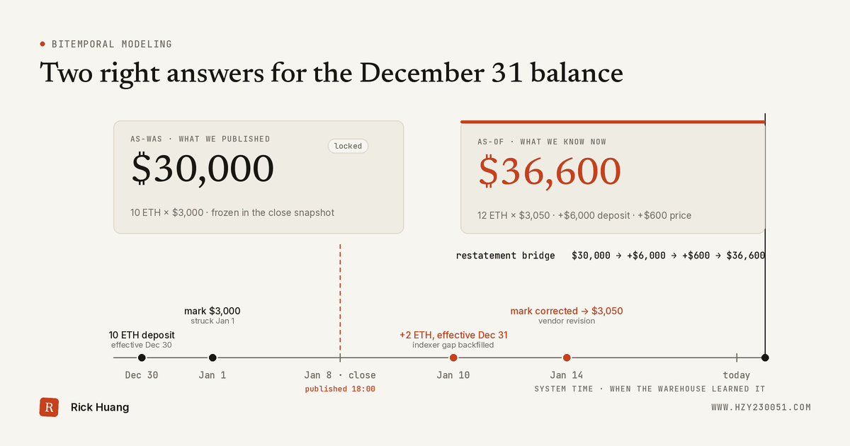
It’s audit season. Somewhere an auditor is holding a December 31 balance from the January close package. Meanwhile someone on the finance team is looking at a dashboard that shows a different December 31 balance for the same account. Nobody made a mistake. A deposit confirmed late and a price vendor corrected a print. Both numbers are right. They answer different questions, and the warehouse has to be able to produce either one on demand and say which one it’s showing.

That’s what bitemporal modeling is for. It sounds academic, but in finance it’s the difference between “we can explain every change since we published” and “the number moved, and we’re not sure why.”

Two clocks

Every financial fact has two timestamps.

Valid time (effective_at) is when the economic event happened: the deposit hit the chain, the trade executed, the price was struck.

System time (recorded_at) is when the warehouse learned about it.

Most of the time they are seconds apart and nobody cares. The interesting cases are when they aren’t, because then “the balance on December 31” splits into two questions:

• As-of: what is our best knowledge today of the December 31 balance?
• As-was: what did we report for December 31 when we closed the books on January 8?

Finance needs both. As-of is for analysis, trends and anything forward-looking. As-was is for anything already published: board decks, client statements, regulatory filings, the numbers the auditor has in hand.

In the ledger-first architecture I described in January, the ledger table already carries both timestamps. This post is about what you do with the second one.

Where the second clock comes from

At a crypto custodian, the gap between valid and system time opens up in predictable places.

Late or corrected prices. The reporting cutoff mark arrives late, or the vendor revises a bad print days later.

Late chain confirmations. An indexer falls behind, a node is down over a holiday, or a deposit sits below the finality threshold across midnight. The transfer happened on December 31; we learn about it on January 10.

Backdated adjustments. Operations discovers a misbooked fee and posts the correction effective in the prior period.

Dimension changes. An account is reclassified from retail to institutional, or two client records are merged. The facts didn’t change, but the grouping they roll up into did.

The pattern

Facts are append-only and carry both timestamps

Nothing is updated in place. A correction is a reversal plus a re-booking, each with its own recorded_at. That alone makes the fact table bitemporal: filter on recorded_at and you get exactly what the warehouse knew at any moment.

Prices follow the same rule. A corrected mark is a new row for the same (asset_id, price_at) with a later recorded_at, never an overwrite.

Dimensions version on system time

Dimensions, the descriptive tables such as accounts and clients, are versioned as SCD2 (slowly changing dimension, type 2) on system time. Every change adds a new row with recorded_from and recorded_to instead of overwriting the old one. Valid-time attributes, such as “this account has been institutional since January 1,” live inside the row as ordinary columns. To see a dimension as it was known at time k, join on recorded_from <= k and (recorded_to is null or recorded_to > k).

I version on system time rather than valid time because the question the auditor asks is “what did you know when you published?” A reclassification recorded in February, effective January 1, must not change the January close package.

One macro answers both questions

-- macros/as_known_at.sql
-- valid_before and known_at are SQL expressions:
--   "timestamp '2025-01-01 00:00:00'"  or  "current_timestamp()"
-- known_at = now gives the as-of answer; known_at = the close gives the as-was one.
{% macro as_known_at(relation, valid_before, known_at) %}
  (
    select *
    from {{ relation }}
    where effective_at <  {{ valid_before }}
      and recorded_at  <= {{ known_at }}
  )
{% endmacro %}

The valid-time bound is half-open on purpose. effective_at <= '2024-12-31 23:59:59' silently drops anything at 23:59:59.4, and chains produce timestamps with sub-second precision all the time.

Close writes a snapshot

At period close, I materialize the as-was result into an immutable close_snapshot table, keyed by period_id and close_version, with the known_at timestamp and the dbt commit stored alongside. Published dashboards and client statements read from the snapshot, never from live models.

A restatement report explains the difference

The last piece is a report that diffs as-was against as-of, by account and by cause. That’s the worked example.

A worked example: one account, one quarter-end

Toy client account C-100 holds ETH at the custodian. The reporting period is Q4 2024, so valid_before is 2025-01-01 00:00:00 UTC. The Q4 close was published on January 8 at 18:00 UTC.

Fact	effective_at	recorded_at
Deposit 10 ETH	2024-12-30 14:05	2024-12-30 14:20
Deposit 2 ETH (indexer gap, backfilled)	2024-12-31 23:41	2025-01-10 09:00
ETH cutoff mark $3,000	2025-01-01 00:00	2025-01-01 00:05
ETH cutoff mark corrected to $3,050	2025-01-01 00:00	2025-01-14 16:30

On the two clocks it looks like this:

system time →   Dec 30    Jan 1    Jan 8 18:00   Jan 10   Jan 14    today
                │         │        │             │        │         │
10 ETH deposit  ●───────────────────────────────────────────────────────▶
2 ETH deposit                      │             ●──────────────────────▶
cutoff mark               ● $3,000 ───────────────────────● $3,050 ─────▶
                                   ▲                                ▲
                                 as-was                           as-of

The query that values the account for any pair of clocks:

{% set valid_before = "timestamp '2025-01-01 00:00:00'" %}
{% set known_at     = "timestamp '2025-01-08 18:00:00'" %}  -- or "current_timestamp()"

with bal as (
  select account_id, asset_id, sum(amount_native) as qty_native
  from {{ as_known_at(ref('fct_ledger_entry'), valid_before, known_at) }}
  group by account_id, asset_id
),
px as (
  select asset_id, price_usd
  from {{ ref('fct_price_mark') }}
  where price_at = {{ valid_before }}
    and recorded_at <= {{ known_at }}
  qualify row_number() over (partition by asset_id order by recorded_at desc) = 1
)
select
  b.account_id,
  b.asset_id,
  b.qty_native / a.unit_scale                as qty,
  px.price_usd,
  b.qty_native / a.unit_scale * px.price_usd as value_usd  -- NULL if no mark was known yet
from bal as b
join {{ ref('dim_asset') }} as a using (asset_id)
left join px using (asset_id)

Run it twice and you get the two answers:

View	known_at	Quantity	Mark	Value
As-was (published close)	2025-01-08 18:00	10 ETH	$3,000	$30,000
As-of (today)	now	12 ETH	$3,050	$36,600

Neither is wrong. The client statement that went out in January said $30,000 and should keep saying so. The analyst modeling year-over-year growth should use $36,600.

The restatement bridge

A $6,600 gap with no explanation is how trust in a finance team erodes. The restatement report breaks it down by cause:

Step	Amount
As-was, published January 8	$30,000
Late deposit: 2 ETH at the original $3,000 mark	+$6,000
Price correction: 12 ETH × $50	+$600
As-of, today	$36,600

The order of attribution is a convention, and you have to pick one. I value quantity changes at the old price first, then apply the price change to the new quantity. Reverse it and you get $500 of price effect and $6,100 of quantity effect. Both sum to $6,600. What matters is that the convention is written down and never changes between quarters.

The quantity side of the bridge comes from a simple query: every fact that belongs to the period but arrived after the close.

select
  account_id, asset_id, event_type, source_system,
  count(*)            as late_entries,
  sum(amount_native)  as qty_native_delta
from {{ ref('fct_ledger_entry') }}
where effective_at <  timestamp '2025-01-01 00:00:00'
  and recorded_at  >  timestamp '2025-01-08 18:00:00'
group by account_id, asset_id, event_type, source_system

Grouping by source_system is what turns this from a number into a diagnosis. If every late entry came from one chain indexer, that’s an operational fix, not an accounting one.

Whether a late item gets restated or booked as an adjustment in the current period is a materiality judgment for the accountants, not a data decision. The model’s job is to make the size and cause of every change obvious, so that judgment takes minutes instead of days.

Trade-offs

Storage and cost. Keeping every version is cheaper than it sounds. The ledger is append-only anyway, and price corrections are rare. The real cost is query complexity: every join to a dimension now needs a system-time predicate. I partition facts by date(effective_at) and cluster by account, which keeps period queries cheap whatever known_at is.

Snapshots vs. reconstruction. In theory, the macro alone can reproduce any as-was number, so why snapshot? Because there’s a third clock: the code. If someone fixes a bug in the balance model in February, replaying the January close with February’s code gives a different answer even though no data changed. A snapshot captures data and logic together, and that is what an auditor can rely on. I treat reconstruction as a check against the snapshot, not a replacement for it.

When not to bother. Most product analytics doesn’t need any of this. Funnel conversion for last Tuesday is fine as-of. Bitemporality earns its keep where numbers get published and someone can later ask why they changed: balances, revenue, fees, anything client-facing or regulatory.

What goes wrong in practice

recorded_at means load time. If a source is backfilled or migrated, every row gets today’s load timestamp and the restatement report lights up with years of “late” facts. For initial loads, I take the source’s own creation timestamp where it’s trustworthy and flag the row as recorded_at_inferred. After that, recorded_at is the first time the pipeline saw the row, and it never changes.

Mutable sources. If an upstream system overwrites rows in place, system time is lost the moment you sync it. Staging has to capture changes, via change data capture (CDC) or dbt snapshots, or the second clock simply doesn’t exist for that source.

Time-zone cutoffs. A December quarter that ends at midnight New York time ends at 05:00 UTC. If the macro gets a UTC midnight and the price mark is struck in Eastern time, every quarter has a five-hour sliver of disagreement.

Dashboards on live models. The most common failure isn’t technical. Someone builds the board dashboard on the as-of model because it’s “more accurate,” and Q4 revenue changes in March, in front of the board. Anything published reads from the snapshot.

Dimension joins without a system-time predicate. One forgotten predicate and the as-was report quietly regroups history under February’s account hierarchy. I add a test that recomputes each close snapshot’s totals by segment and fails if they drift.

Label which answer you’re showing

Bitemporal modeling doesn’t make the data more correct. It makes it accountable. Every number in the warehouse can say both what happened and when we knew it, and those are separate claims.

The practical rule I hold teams to is simple: every finance chart and table states whether it is as-of or as-was, and every as-was number links to the close snapshot it came from. When the two disagree, the restatement report explains why in one table. That’s a conversation an auditor is happy to have.